 “A Pinch of Probability is worth a pound of Perhaps” – James Thurber.
This quote is more true today than it was when James originally wrote it in 1961.
In today’s complex world the proper understanding and application of Probability will allow you to maximize your impact on Quality.
Maximizing your impact on quality requires focus on the most important problem.
Focusing on the most important problems starts by identifying the highest risk areas within your business that truly require your attention.
The concept of Probability gives us a tool that can be used to identify these high risk areas that require attention.
Recall that the risk associated with any given failure mode is: Risk = Probability * Severity
This chapter is dedicated to Probability, and specifically the following areas:
- Terminology – Define and apply quantitative terms, including population, parameter, sample, statistic, random sampling, and expected value. (Analyze)
- Probability terms and concepts – Describe concepts such as independence, mutually exclusive, multiplication rules, complementary probability, and joint occurrence of events. (Understand)
If you’re following along with the 2015 CQE Body of Knowledge, you’ll notice I’ve excluded a portion of the body of knowledge from this chapter:
Drawing statistical conclusions – Distinguish between numeric and analytical studies. Assess the validity of statistical conclusions by analyzing the assumptions used and the robustness of the technique used. (Evaluate)
Instead of discussing this topic here, I thought it was a better fit within the previous chapter on Collection & Summarizing Data – Part 2.
Probability Terminology
Alright, let’s jump right in.
We will start with the basic terms & definitions and then move into more complex topics.
There are five key definitions to cover – Probability, Experiment, Outcome, Sample Space & Event.
Let’s start with Probability which is defined as the likelihood (or chance) that an event will occur.
Probability is normally expressed as a Percentage (%) or Decimal (0.0 – 1.0).
Below I’ll show you how to calculate probability, but before that let’s make it through these definitions.
As we move through this section you’ll see all of the common probability examples – the coin flip, the dice roll, a random card pulled from a deck of 52 cards.
These are all examples of our next definition, what statisticians call an Experiment.
In an experiment there is a fixed number of outcomes where the probability of each outcome can be calculated.
An outcome is defined as the result of an experiment.
For example, the experiment of flipping a coin has two possible outcomes; heads or tails.
The experiment of rolling a 6-sided dice has 6 possible outcomes; 1, 2, 3, 4, 5, 6.
A full deck of cards has 52 cards, where each card is considered a unique outcome when pulling 1 card randomly.
This leads us to our next definition – sample space.
In the coin flip & dice roll examples above I listed out all possible outcomes within that experiment.
This total collection of all possible outcomes is known as the sample space of an experiment.
This sample space is usually denoted as “S” along with brackets like this S{1,2,3,4,5,6} for the dice role experiment or S{H,T} for the coin flip experiment.
One key thing to remember about the sample space is that the probability of all outcomes within a sample space must add up to 1 – let’s see what this looks like for the dice roll.
P(Sample Space) = P(1) + P(2) + P(3) + P(4) + P(5) + P(6) = 1.00 = 100%
If you’ve truly defined the entire sample space for an experiment, the probability of all of the individual outcomes within that experiment must add up to 1 or 100%.
Let’s move on to the next definition, an Event.
Similar to a simple outcome (flipping a heads), an event is defined as a single outcome or collection of outcomes that might occur during an experiment.
Events are generally more complex than a simple outcome because they often reflects a collection of outcomes.
Let’s jump back to our first definition, Probability, and look at a few examples.
Probability Example 1 – The Dice Roll
What is the probability of rolling a six sided dice and getting a 4 (Event A)?
There are 6 possible events that can occur when you role a six sided dice.
Rolling a 4 represents one of those 6 possible events.
Therefore the probability is 1 in 6 or 1/6, which is equal to 0.167 or 16.7%.

Let’s quickly review the terms & definitions above to help you calibrate:
Experiment: Rolling a Dice
Sample Space: The entire sample space can be defined by the potential outcomes, rolling a 1, 2, 3, 4, 5 or 6.
This sample space forms the denominator of the probability calculation above as there are 6 potential outcomes.
Event: The event in this experiment is a simple outcome, rolling a 4.
Let’s see another example with a more complex Event.
Probability Example 2 – The Dice Roll, Take 2
An example of a more complex event within the dice roll experiment is a roll of an even number which is a collection of 3 outcomes {2,4,6}, let’s call this Event A.

Or another event within the dice roll experiment could be any number higher than 2 {3,4,5,6}, which is a collection of 4 possible outcomes, let’s call this Event B.

Probability Example 3 – Flipping 2 Coins
Another common example I’ll use now is the experiment of flipping 2 coins simultaneously.
What is the probability of flipping only 1 heads (Event A)?
Let’s start by defining our sample space for this experiment.
So there are 4 possible outcomes when flipping 2 coins simultaneously:
- HH: Heads/Heads,
- HT: Heads/Tails,
- TH: Tails/Heads,
- TT: Tails/Tails
Thus our sample space consist of 4 possible outcomes S{HH, HT, TH, TT}.
There are only 2 outcomes within the sample space that fall within Event A (only 1 heads); these are HT & TH.
Now let’s use the probability calculation to get our final answer:

Probability Example 4 – Random Sampling from a Jar
Now let’s get a little more complex with it and I’ll show you how you can use a tool like a tree diagram to help you solve a probability problem.
Let’s say you’ve got a jar that full of black and white marble that are evenly distributed; so 50% white marble, 50% black marbles, and you want to sample 3 marbles randomly from that jar.
Here’s how a tree diagram can help you determine your sample space for this experiment:

In the image above we’ve taken 3 samples and used the tree diagram to accurate define our sample space which is 8 total outcomes.
Now let’s use this example to determine the probability of event A, which is defined as all outcomes where only 1x black marble is sampled.
So if we go back to our tree diagram, we can find 3 outcomes that are associated with only 1x black marble being sampled.

Now we can calculate the probability!

This is all based on the assumption that the black and white marbles are evenly distributed within the jar and that at any given time there is a 50/50 chance of drawing either a black or white marble.
Compound Events
Alright, let’s go even deeper into the world of probability by discussing compound events.
Up until now we’ve talked about some fairly simple events, the single coin flip & the single dice roll.
However oftentimes in probability we’re interested in calculating the probability of compound (multiple) events.
These methods & tools will help you analyze any complex situation you might encounter as a Quality Engineer; and be able to estimate probabilities of occurrence.
There are 3 Compound Events to discuss, the Union, the Intersection & the Complement.
Before we jump in let’s discuss a new tool we’re going to use, the Venn Diagram.
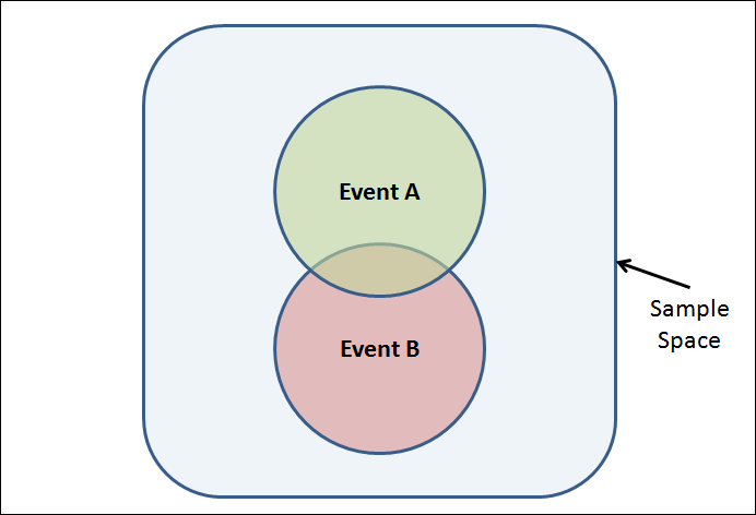
Below is a simple Venn Diagram, which shows the entire sample space of an experiment in blue, and two Events, A & B, within that sample space.
Oftentimes, as in the diagram below, two events will overlap each other. This means that those two events share common outcomes between them.
The Venn Diagram will be used throughout this section to assist you in understanding the 3 Compound Event Functions – Unions, Intersections & Complement.
 The Union of Multiple Events
The 1st Compound Event within Probability is the Union.
The union of multiple events is the combination of all of the possible outcomes contained within those multiple events.
The union is denoted as and should be read as “A or B”, and let’s jump right into an example.
Union Example A – Deck of Cards
In this example, the experiment is picking 1 card randomly from a standard deck of 52 cards, where two events (A & B) have been defined and we’d like to know the probability of either of them occurring.
Event A – Picking a Spade (13 out of 52) – (A, 2, 3, 4, 5, 6, 7, 8, 9, 10, J, Q, K).
Event B – Picking a Face Card (12 out of 52) – (J, J, J, J, Q, Q, Q, Q, K, K, K, K).
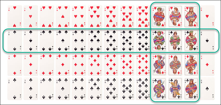
The union of those two events would be the probability of picking a random card that was either a spade OR a face card.
The Union of Event A & B then becomes the following cards – (A, 2, 3, 4, 5, 6, 7, 8, 9, 10, J, Q, K, J, J, J, Q, Q, Q, K, K, K)
Notice here that these two events share some outcomes, namely the Jack, Queen & King of Spades – more on handling this below.
So the Union of A & B (A U B) allows you to determine the probability of picking a spade OR a face card. This can be seen in the Venn Diagram Below, where on the left the two separate events can be shown.
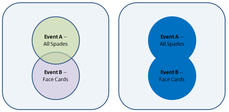
The Union of these two events can be seen in the image on the right. The overall probability of either event occurring can be thought of as the probability of any outcome within the blue shaded region occurring.
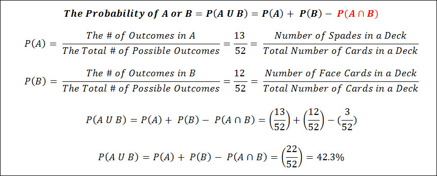
As a segue into the next topic I wanted to point out the back half of that equation, P(A ꓵ B).
This portion of the equation is known as the Intersection between two events.
The intersection is subtracted from the Union equation to prevent double counting of these outcomes. as the probability of drawing these cards is already captured in the Probability of Event A, P(A).
This is the Jack, Queen & King of Spades, which are the outcomes we discussed above that are associated with both events A & B. Let’s dive into the topic of intersections now so you can see how I calculated that value.
The Intersection of Multiple Events
The 2nd Compound Event within Probability is the Intersection.
The Intersection of two events (A & B), is the collection of all outcomes that are common between the two events.
This function determines the overlap between 2 events.
The Intersection of two events is denoted by the symbol ꓵ & looks like A ꓵ B, which is read as the Intersection of A & B.
Intersection Example A – Deck of Cards
In this example above the experiment is picking 1 card randomly from a standard deck of 52 cards, where two events (A & B) have been defined.
Event A – Picking a Spade (13 out of 52) – (A, 2, 3, 4, 5, 6, 7, 8, 9, 10, J, Q, K).
Event B – Picking a Face Card (12 out of 52) – (J, J, J, J, Q, Q, Q, Q, K, K, K, K).
Where the Intersection of A & B (A ꓵ B) would allow you to determine the probability of picking both a spade and a face card.
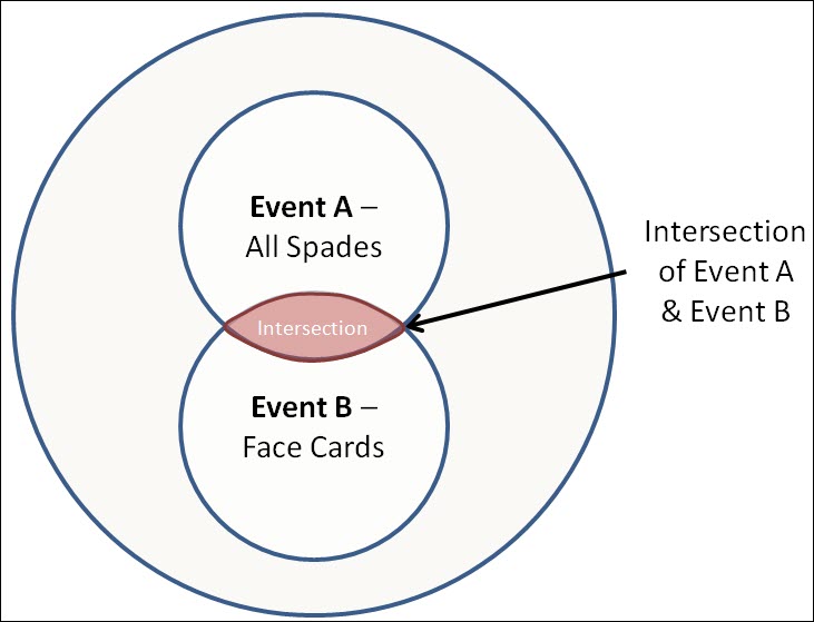
The Intersection of Event A & B would be the probability of picking a random card that was either a spade or a face card, so the Jack, Queen & King of Spades.
So the Probability of both events occurring:
P(A ꓵ B) = P(Jack of Spades) + P(Queen of Spades) + P(King of Spades) =
P(A ꓵ B) = (1 / 52) + (1 / 52) + (1 / 52)
P(A ꓵ B) = (3 / 52) = ~6%.
Intersection Example B – The Dice Roll
The other example of an intersection is the dice roll.
The single dice roll has the following sample space S{1,2,3,4,5,6} and two events have been defined:
Event A has been defined as a roll that comes up with an even number, so A{2,4,6}.
Event B has been defined as a roll that comes up less than 4, so B{1,2,3}.
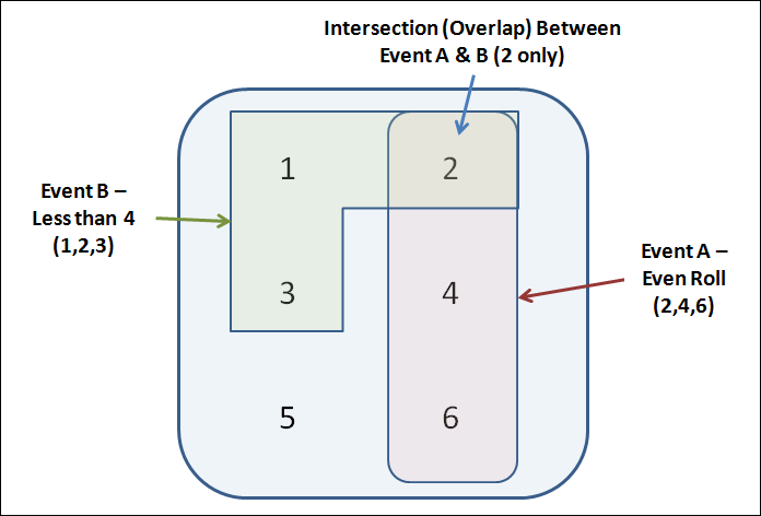
So the Intersection of A & B, denoted as A ꓵ B = (2, 4, 6) ꓵ (1, 2, 3) = (2)
P(A ꓵ B) = P(2) = 1 / 6 = ~17%.
Based on the definition of an intersection, the only common outcome shared between these two events is a 2, and the probability of a roll of 2 is 1 out of 6.
This can be interpreted as, 1 in 6 dice rolls would result in both events occurring.
The Complement
The Complement of Event A, usually denoted as A° or A’, is a combination of all outcomes of the sample space that are not captured within Event A.
The complement of A is essentially the opposite of A.
Because the Complement of A captures all other outcomes in the sample space that are not captured within Event A; then the combination of A & A° captures the entire sample space.
This can be expressed in the form or The Complement Rule Equation:

You can visualize the Complement in the Venn Diagram below – the Complement is essentially all of the sample space that’s not captured by Event A.
Here we’ve taken a deck of 52 cards and defined Event A as a single card pulled from the deck coming up as a Spade.
The Complement to this Event would be any suit other than Spades – which includes Diamonds, Hearts & Clubs.
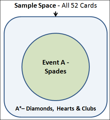
In the example above, the probability of pulling a spade from a random deck of 52 cards is 25%; and the probability of the Complement of A (Diamond, Heart or Club) is 75%.
Complex Probability Concepts
Now that we’ve covered the compound events within probability (Union, Intersection & Complement), it’s time to take our understanding to the next level and introduce some new concepts.
In the examples above for Unions & Intersections we were calculating the probability of those Unions & Intersections.
However these were straight forward examples; and as complexity grows we must understand the concept of Mutual Exclusivity & Independence to accurately calculate probability.
These concepts have an impact on the way we calculate the probability of Compound Events where multiple events are occurring with various potential outcomes.
Within this section we will also cover 3 concepts – Conditional Probability, the Addition Rule & the Multiplication Rule.
The Addition & Multiplication rules combine our knowledge of Unions/Intersections with the concepts of Mutual Exclusivity & Independence to show us how to calculate probability for any given situation.
Let’s start with Mutual Exclusivity.
Mutual Exclusivity
Within probability, Mutual Exclusivity is the concept that two events cannot occur at the same time.
There are simple outcomes that are good examples of this principle.
A coin flip of heads is mutually exclusive from the result of tails.
Rolling a dice and getting an even number is mutually exclusive from getting an odd number.
Other examples can be gleaned from a deck of cards.
For example if you had two events where Event A was all Spades in the deck, and Event B was all Red cards, these two events are mutually exclusive – they cannot occur at the same time.
Mutual Exclusivity is important to probability because it implies that there is no intersection between two events that are mutually exclusive.
Remember the intersection is the combination of all outcomes that are shares between two events.
When two events are mutually exclusive, they do not share any outcomes, thus their intersection is zero.

This fact will help us out later when we talk about Conditional Probability, The Addition Rule & The Multiplication Rule.
Conditional Probability
Alright, now were on to one of the more complex operations within probability that allows us to play the “what if” game.
This “What If” analysis tool is the Conditional Probability concept.
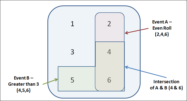
Let’s use the example of the dice roll to illustrate this, and let’s say we’ve got two events, A & B that are:
Event A – An Even Number; {2,4,6}
Event B – Greater Than 3; {4,5,6}
The probability of Event A occurring is 3 out of 6, or 50%. Event B has the same probability.
Now, let’s say we’ve run the experiment (rolled the dice) and what if I told you that Event B had occurred, what is the new probability that Event A has occurred?
This is a Conditional Probability problem.
The conditional probability of Event A, given that Event B has occurred is written as P(A|B), and is the probability that A has occurred when it is already known that Event B has already occur.

Let’s solve the example above using this equation; and we can start by calculating the probability of A & B individually.
A = {2,4,6}, and therefore P(A) = P(2) + P(4) + P(6) = 3/6 = 0.50
B = {4,5,6} and therefore P(B) = P(4) + P(5) + P(6) = 3/6 = 0.50
Remember the Intersection between these two events are the outcomes shared by both Events, which include the 4 & 6, therefore the probability of the intersection is 2 out of 6 or 1/3.
P ( A ꓵ B) = P(4) + P(6) = 2/6 = 0.33
Now we can plug these numbers into the Conditional Probability Formula:

So let’s go back to the word problem itself and make sure we’ve got the conclusion correct.
The probability of Event A (2, 4 or 6) occurring, given that Event B (4, 5 or 6) has occurred is 0.66 or 66%. You can see this in the venn diagram below.
So if I told you that Event B had occurred, there are only 3 possible results (4,5, 6) & two of those outcomes overlap (intersect) with Event A (4 & 6), making the final probability 2/3.
Conditional Probability Example B
Let’s use a deck of cards now for this example, where 2 events have been defined, and we’d like to know the probability of Event A occurring, given that B has already occurred.
Event A – The card drawing is the King of Spades {K of Spades}
Event B – The card drawn is a Face Card (J, J, J, J, Q, Q, Q, Q, K, K, K, K)
P(A) – The Probability of A = 1 in 52 or 1.9%
P(B) – The Probability of B = 12 in 52 or 23.1%
Remember the Intersection between these two events are the outcomes shared by both events which in this case only includes the King of Spades.
P ( A ꓵ B) = P(King of Spades) = 1 in 52
Now we can plug these numbers into the Conditional Probability Formula to see what happens to the Probability of Event A, given that Event B has occurred:

You can think of this example as I removed all non-face cards from the deck, which would leave us with 12 cards total, and then I asked you what the probability of drawing the king of spades would be – which is 1 in 12.
Independence
The idea of conditional probability above tells us that there are certain situations when the occurrence rate of the first events (B) results in a change of the probability of occurrence the 2nd event (A).
Is it possible to have two events, where the occurrence of the 1st event does not change the probability of the 2nd event occurring?
Sure it is!
This is the concept of Independence.
Two events are independent if the occurrence of one event does not change the probability of occurrence of the other event.
Let’s see what this looks like from a mathematical perspective by starting with the end in mind – and seeing what happens to the conditional probability equation when we’re dealing with two independent events.
So we know from above chapter on Conditional Probability that the probability of A, Given that B has occurred can be calculated using the following equation:

Now let’s look at what has to happen for P(A|B) to equal P(A), because when these two are equal, it implies that the occurrence of B had no effect on the occurrence of A.
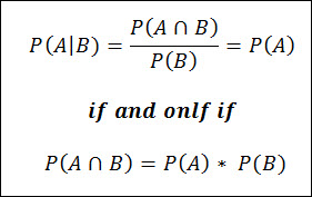
So, if the intersection of A & B, P(A ꓵ B), is equal to the Probability of A multiplied by the Probability of B, then the Conditional probability of A given that B has occurred will simply be equal to the Probability of A.
Let’s plug this intersection back into the original conditional probability equation to show this.

Based on this we can confirm then that – 2 Events are only independent if and only if P(AꓵB) = P(A)*P(B).
IF P(AꓵB) ≠ P(A)*P(B), then A & B are not Independent (they are dependent).
When two events are independent, then the Probability of A AND B occurring, denoted as P(AꓵB), is calculated as such:

This is an important topic in probability because it allows us to estimate the occurrence rate of multiple independent events all occurring at the same time, which is extremely useful in the Risk Management process.
 Example – Intersection of Independent Events
For example, let’s say that you’ve got a visual inspection for a critical failure mode, and let’s say this visual inspection actually occurs 2 times by 2 different independent operators – so a 200% inspection.
Let’s also say that this critical failure mode occurs on 1% of product, and the detection rate during the visual inspection is 80%.
What is the probability that a critical failure mode is produced and then subsequently goes undetected in the 200% visual inspection.
Event A – Occurrence of a Critical Failure Mode – 1%
Event B – Non-detection of the failure mode by 1st inspector – 20%
Event C – Non-detection of the failure mode by 2nd inspector – 20%.
Assuming that these 3 events are independent, we can then use the equation below to estimate that probability:

At this probability, the occurrence rate of a critical defect that goes undetected is approximately 1 in 2,500.
Then from a risk management perspective you should compare this occurrence rate against the severity of the failure mode to analyze the overall risk.
The Addition Rule in Probability
In the section above for Unions we learned how to take two events and combine them into a Union which would allow us to calculate the probability of either event occurring.
The Addition Rule is the probability tool used to calculate the probability associated with a union of two or more events.
Recall now that a union is analogous to the EITHER/OR function.
That is, either event A can occur OR event B can occur OR both events can occur – in either situation the Union of those two events would occur.

Above is the Addition Rule which states that the probability of the union of 2 or more events (A, B, etc) can be calculated by adding the probabilities of each event, P(A), P(B), etc, and then subtracting the intersection between those 2 events, P(A ꓵ B).
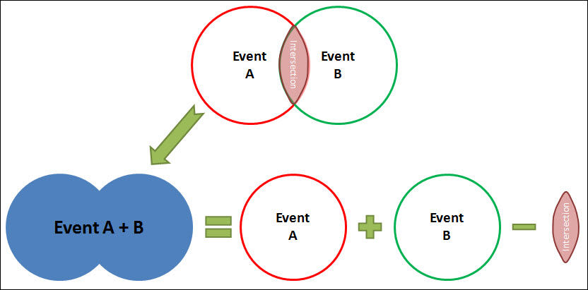
Essentially, the probability of either A or B occurring is the probability of A, plus the probability of B minus the probability of both occurring.
Addition Rule for Mutually Exclusive Events
Recall that for mutually exclusive events, the intersection between events is zero:

Therefore, for events that are mutually exclusive the Addition Rule above simplifies to:

The Multiplication Rule in Probability
Alright, on to the last topic within Probability – the Multiplication Rule.
The Multiplication Rule allows you to calculate the probability that 2 different events or outcomes will both occur.
This is analogous to the AND function where both events MUST occur.
This is different from the Addition Rule which allows you to determine the probability that either of two events will occur.
To fully understand the multiplication rule, we must apply all of the information we’ve learned above.
This includes our knowledge of Independence, Conditional Probability and the Intersection of dependent events.
Multiplication Rule for Independent Events
For example, the probability of 2 independent events both occurring looks like this:

For example if you had two independent events:
Event A – Rolling an even number – where the probability of A is P(A) = 3 out of 6 or 0.50.
Event B – Flipping a Tails – where the probability of B is P(B) is 1 out of 2 or 0.50.
So the odds of rolling a dice and flipping a coin where the outcome was both tails and an even roll is:

This is the straight forward version of the multiplication rule.
The rule becomes a bit more complicated with the 2 events in question are dependent events.
Multiplication Rule for Dependent Events
This is where our knowledge of conditional probability comes into play.
Recall our discussion on Conditional Probability above where the Probability of A, given that B has already occurred looks like this:

This equation can be rearranged to form the multiplication rule for dependent events:

Let’s see what an example looks like – let’s say we’ve got a jar with 4 different color marbles of the following quantity:
- 20 black marbles
- 10 white marbles
- 15 green marbles
- 5 blue marbles
So 50 marbles in total.
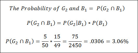
Let’s say that I asked you to calculate the probability of sampling a blue marble on your first random attempt and then a green marble on your 2nd attempt, and we’re not replacing marbles after sampling.
Event B1 – 1st Marble is Blue- B1
Event G2 – 2nd Marble is Green – G2
Because we’re sampling without replacement, these 2 events become dependent as the results of the 1st sample have an impact on the probability of the second sample.

Where the probability of the 1st marble being blue is:

Then, we must calculate the probability of the 2nd sample being green.
With this 2nd sample we know that there are now 49 total marbles in the jar, with 15 of them being green, so we can calculate the probability of that 2nd sample being green.

Notice here how the denominator is 49 and not 50. This is because it’s the 2nd sample and we’ve already pulled 1x marble from the jar that was not a green marble.
Now we can calculate the probability of the 1st marble being blue, and the 2nd marble being green.
Conclusion
Alright – let’s recap everything we learned.
Terminology
We started by covering the basic definitions within probability: Probability, Experiment, Outcome, Sample Space & Event.
Probability is defined as the likelihood (or chance) that an outcome or event will occur. Probability is normally expressed as a Percentage (%) or Decimal (0.0 – 1.0).
An outcome is defined as the result of an experiment.
Similar to an outcome, an event is defined as a single outcome or collection of outcomes that might occur during an experiment.
Within an experiment it’s important to understand the sample space which is defined as a collection of all possible outcomes within that experiment.
Compound Events
From here we went deeper into the world of probability by discussing 3 compound events – the Union, the Intersection & the Complement.
The union of multiple events is the combination of all of the possible outcomes contained within those multiple events. The union is denoted as and should be read as “A or B”.

The Intersection of two events (A & B), is the collection of all outcomes that are common between the two events and allows us to determine the overlap between 2 events.
The Intersection of two events is denoted by the symbol ꓵ & looks like A ꓵ B, which is read as the Intersection of A & B.

The Complement of Event A, usually denoted as A° or A’, is a combination of all outcomes of the sample space that are not captured within Event A.

Complex Probability Concepts
Next we went even deeper into probability and discussed the concepts of Mutual Exclusivity & Independence, which we learned are concepts which we must use to determine the proper Addition & Multiplication equation.
Mutual Exclusivity is the concept that two events cannot occur at the same time. 
We also learned that two events are independent if the occurrence of one event does not change the probability of occurrence of the other event.
Within this section we will also cover 3 probability tools – Conditional Probability, the Addition Rule & the Multiplication Rule.
Conditional Probability allows us to calculate the probability of occurrence of multiple dependent events.

The Multiplication rule combines our knowledge of Intersections, Conditional Probability, & Independence to show us how to calculate the probability of two events occurring together.

The Addition rules combines of Unions, Intersections, & Mutual Exclusivity to show us how to calculate the probability of the union of two events occurring.


