Acceptance Sampling is a practice whereby a sample is tested from a population (lot), and a decision to accept or reject that entire population (lot) is based on the test results of the sample.
Acceptance Sampling originated in the 1930’s at Bell Labs through the work of Harold Dodge and was later popularized during World War II by the U.S. Military for munitions (bullets) production.
During the war, many bullets were produced and there was no economic way to test them all. Additionally, some of the testing was destructive, rendering the munitions unusable, so 100% inspection was impossible.
Acceptance Sampling became the compromise between no inspection and 100% inspection, and allowed the manufacturers to infer the overall “quality” of an entire lot while only testing a fraction of the entire lot.
Over time, acceptance sampling has also become advantageous for other companies who have faced destructive inspection, or when the cost associated with 100% inspection was not economical, or where the risk of passing along a defect is low.
This chapter has 3 major parts:
The First is sampling concepts – This includes topics such as the operating characteristic (OC) curve, producer and consumer risk, and discussion of common sampling terms like AQL, LTPD.
The second part is the sampling standards and plans – This includes a review of ANSI/ASQ Z1.4 and Z1.9 standards, an explanation of single, double, multiple, sequential, and continuous sampling plans.
Third is Sample integrity – Includes a discussion of the techniques for establishing and maintaining sample integrity when executing a sampling plan.
Part 1 – Sampling Concepts
Part 1 is broken up into 3 sub-sections:
- Operating characteristic (OC) curves
- Producer and Consumer Risk
- Terms and Definitions for AQL and LTPD.
These 3 topics are all interrelated, and are foundational to the concept of acceptance sampling.
We will start first with the OC Curve, which will naturally lead us into the risks (producer risk and consumer risk) associated with sampling, then finally the related terms of AQL, LTPD, AOQ and AOQL.
Operating Characteristics (OC) Curves
An OC Curve is a visual representation of how well a specific sampling plan can discern between good and bad lots.
Below is an example of an OC Curve.
The Y-axis is the Probability of Acceptance (Pa), and the curve shows how the probability of acceptance changes depending on the incoming quality level, which is shown on the X-axis.
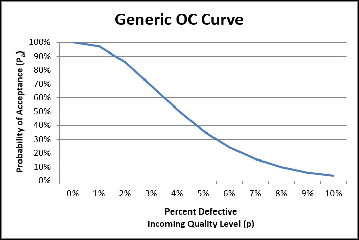
An OC Curve allows you to visually evaluate a sampling plan and understand the probability of accepting a lot of varying quality levels.
The OC Curve for a Perfect Sampling Plan
To understand how an OC Curve works, and its relationship to the risks within acceptance sampling we should with a discussion of the perfect OC Curve.
Let’s say you purchase 100,00 resistors for an electronic product, and your AQL is set at 3%.
The ideal sampling plan would accept all lots with less than 3% non-conformances, and reject all lots with 3% or more non-conformances.
The OC Curve for this ideal sampling plan would look like the one below.
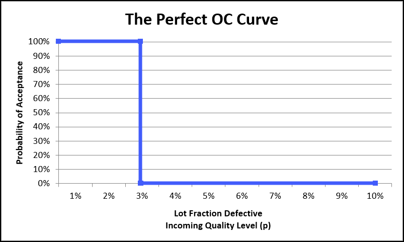
You can see that the probability of acceptance is 100% for all incoming quality levels less than 3% non-conforming, and 0% for all incoming quality levels of more than 3% non-conforming.
This means we will accept any incoming lot whose quality level is less than 3% non-conforming, and reject all lots whose incoming quality level is greater than 3%.
Sampling doesn’t work this way.
Sometimes we accept lots whose quality is poor, and sometimes we reject lots whose quality is good.
These are the risk associated with sampling.
Let’s discuss how to create a OC Curve, and then you’ll be able to visualize the risks associated with sampling.
Creating an OC Curve
OC Curves are constructed through a calculation of the Probability of Acceptance (Pa) for various incoming quality levels (p).
The majority of acceptance sampling plans use attribute data, and this example above is no different.
Because we’re using attribute data, the binomial distribution can be used to calculate the probability of acceptance.
This equation can be executed at various incoming quality levels (p) to construct the entire OC Curve:

Where:
- d = the number of non-conformances observed during sampling
- c = the acceptance number associated with the sampling plan
- n = the sample size associated with the sampling plan
- p = the incoming quality level
OC Curve Example Using the Binomial Distribution
Let’s say you work for a manufacturer executing a sampling plan on a recently received lot of purchased components.
Your sampling plan has you sampling 60 components and you believe the overall percent non-conformance from the purchased vendor lot is 1 percent, and a 99% conformance rate.
You will accept this lot with 1 or fewer defects (c < 1).
What is the probability that fewer than 1 non-conformance (c < 1) will be found in this sample of 60, when the incoming quality level is known to be 1%?

The equation means that the probability that d is less than or equal to 1 (d < 1) is equal to the probability that d = 0 plus the probability that d =1.
We have to calculate each of these probabilities separately, then add them up to find the cumulative probability.

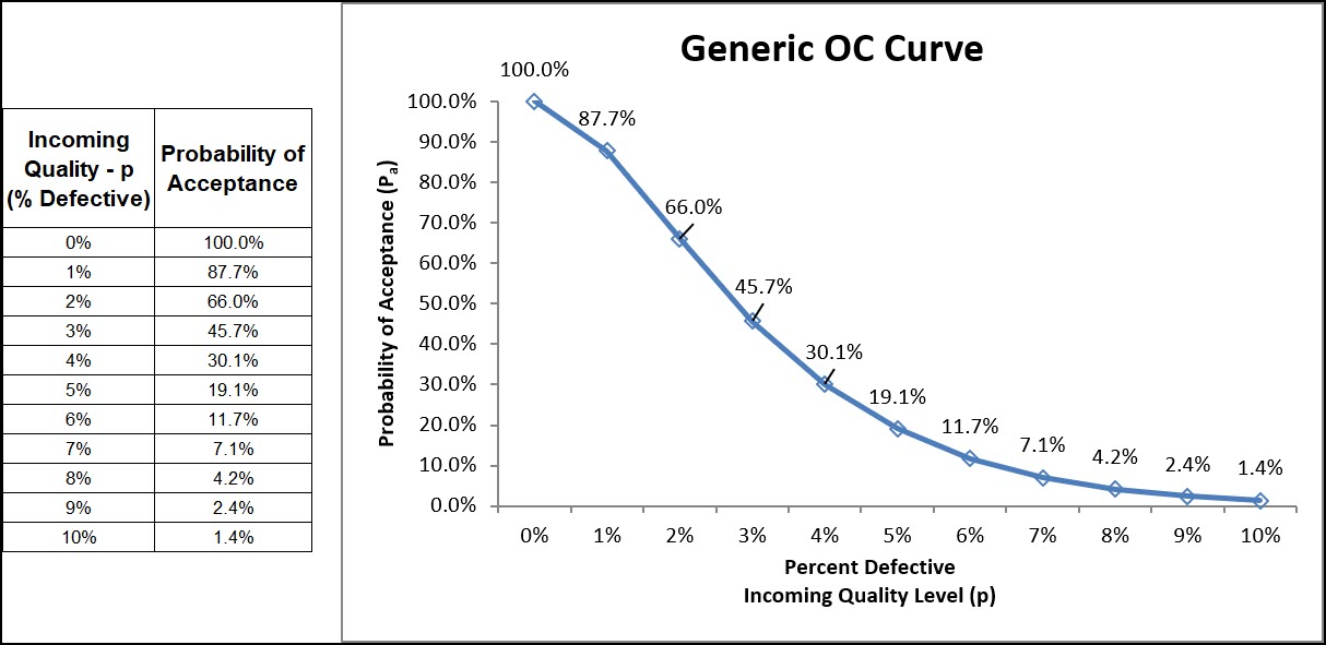
I’ve repeated this calculation for all incoming quality levels (p) and calculated the probability of acceptance to create the entire OC Curve.
The Poisson Approximation
When the defect rate is less than 10%, and the sample size is large, the Poisson distribution is an appropriate approximation for the binomial distribution.
This is often preferred as the calculations are easier, and the Poisson tables are easier to use.
Below is the equation to use to calculate the probability of acceptance using the Poisson distribution.

Where:
- μ = n*p = the sample size multiplied by the incoming quality level
- d = number of non-conformances uncovered in the sample
Essentially what we’re calculating the probability that exactly “d” number of non-conformances are uncovered in a sample of n units, whose incoming quality level is estimated to be “p” in terms of percentage of non-conforming units.
Similar to the Binomial Distribution, the cumulative probability is expressed like this, where c = 1:

Let’s do this math for this specific example, where:
- n = sample size = 60
- p = percent non-conforming of lot being inspected = 1%
- μ = n*p = 60*0.01 = 0.6

As you can see, this probability calculation is nearly identical to the binomial distribution calculation, and is much easier to perform.
Actual OC Curves – Varying Sample Size and Acceptance Number
Sampling plans and their associated OC Curves are defined by two parameters, the Sample Size (n), and the Acceptance Number (c).
The Sample Size (n) is the number of samples to be inspected. The Acceptance Number (c) is the maximum number of non-conformances allowed within the sample.
You’ll also see a rejection number (r), which for single sampling plans, is always one non-conformance more than the acceptance number (c). For double and multiple sample plans this rejection number will vary.
The last parameter of any sampling plan is the number of non-conformances, d, which is the actual number of non-conformances observed in a sample.
- If the sample is taken and d (actual non-conformances observed) are more than the acceptance number (c), then the lot is rejected.
- If the sample is taken and d (actual non-conformances observed) is less than or equal to the acceptance number (c), then the lot is accepted.
Back to Sample Size and Acceptance number – When you change these two parameters, the sample plan and its OC curve changes drastically. Let’s see what this looks!
The OC Curve and Varying Acceptance Number
Let’s start with an example where we hold the sample size constant, and vary the Acceptance Number and let’s see the impact on the sampling plan, its OC Curve, and the probability of accepting a lot.
The example below is for a sample size of 50, with 4 different acceptance numbers (c=0, c=1, c=2, c=3).
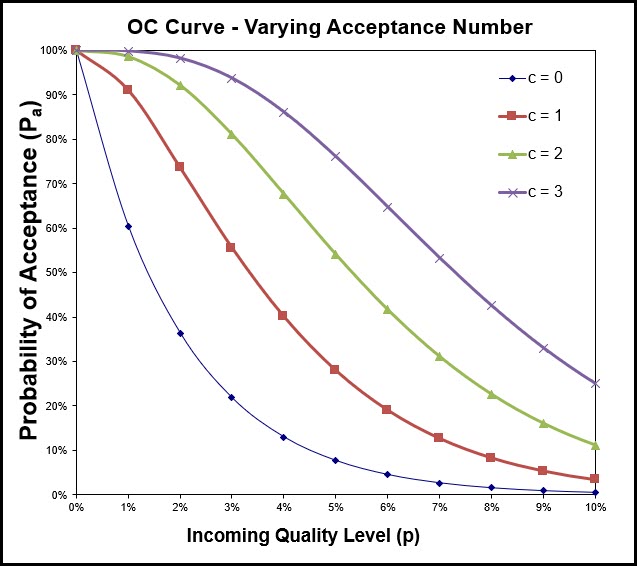
You can see here that having an acceptance number of zero has a much steeper OC Curve than the OC Curve associated with larger acceptance numbers (1, 2 of 3).
Let’s look at the probability of acceptance values below, which are the data points making up the four OC Curves above.
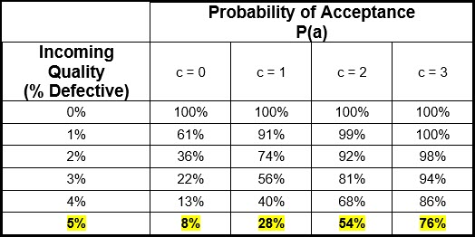
Let’s look at a particular incoming quality level of 5%, where 5 out of 100 units within the lot are non-conforming.
- The probability of sampling 50 units from this lot, and finding zero non-conformance (c = 0 plan), is only 8%.
- The probability of sampling 50 units from this lot, and finding two non-conformance (c = 2 plan), is higher at 54%.
The conclusion here is that a lower acceptance number has a steeper OC Curve, and are much more likely to reject incoming lots with poor quality.
Below we will talk about AQL (Acceptance Quality Limit). You will pick your AQL level for your sampling plan, and this AQL number will dictate your acceptance number.
Smaller AQL values have lower acceptance numbers and thus the sampling plan is more likely to reject lots with poor quality. Larger AQLs have a higher acceptance number and thus have the opposite effect.
The OC Curve and Varying Sample Size
Now let’s hold the acceptance number constant at 1 (c=1), and see what happens to the OC curve when we change the sample size (n). Below are 4 different OC Curves, all at c=1, but with varying sample sizes.
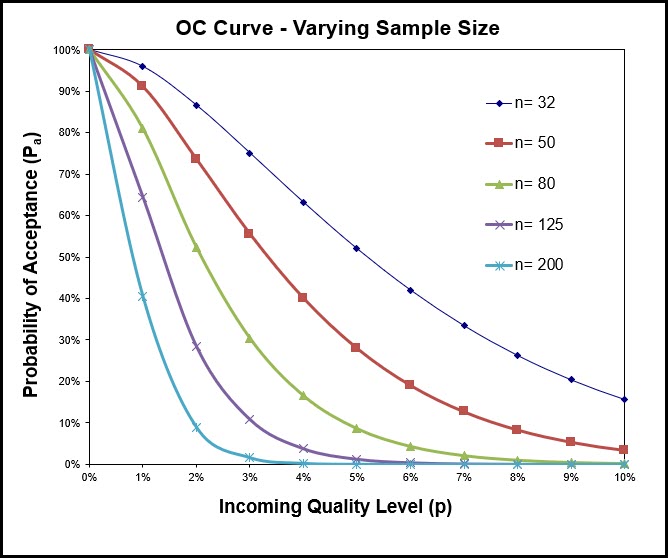
Remember, this sampling plan has an Acceptance Number of 1, this means that if the actual number of non-conformances found during sampling (d) is 2 or more, we reject the whole lot.
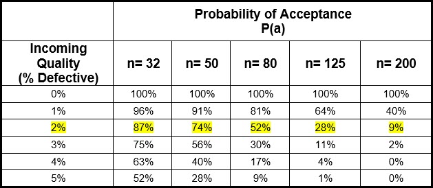
Let’s look at the probability of acceptance for these various sample sizes, with particular attention to the 2% incoming quality level.
- When 200 samples are taken, the probability of accepting a lot with 2% non-conformances is very low, at 9%.
- When only 50 samples are taken, the probability of accepting a lot with 2% non-conformances is much higher, at 74%.
The conclusion here is that sampling more units improves the sampling plans ability to discern between high quality incoming lots and bad ones.
Looking at this table though, you can see that there is still a risk that your sampling plan will not always make the correct accept/reject decision. When our plan does not make the right decision, we introduce some risk into the process.
Let’s now discuss the 2 risks associated with acceptance sampling.
The 2 Risks of Acceptance Sampling
Acceptance sampling is similar to other statistical techniques, specifically those of inferential statistics where we’re taking data from a sample and making inferences about the entire population.
Other topics in inferential statistics include Point Estimates & Confidence Intervals, Hypothesis testing, ANOVA Analysis, etc.
Similar to these other topics in inferential statistics, there’s a chance that sampling might leads us to the wrong conclusion about the overall population.
Producers Risk and Consumers Risk are the terms for these errors in acceptance sampling because Acceptance Sampling is often used when material moves from a producer (seller) to a consumer (buyer).
Remember, the goal of acceptance sampling is to accept good material, and reject bad material. So, two of the four outcomes below are correct.
Producer and Consumer Risk arises when we make the wrong decision.

Producers Risk is the risk (probability) of rejecting a lot whose true quality level meets or exceeds the required quality level (AQL). Producers risk is typically denoted as α, and the most common target for producers’ risk is 5% (0.05).
Consumers Risk is the risk (probability) of accepting a lot whose true quality level does not meets the required quality level (LTPD). Consumers risk is typically denoted as β, and the most common target for consumers risk is 10% (0.10).
For any given sampling plan, the risks associated with that plan (Consumer Risk and Producer Risk) associated with that plan can be seen in the OC Curve along with their relationship to the AQL and LTPD levels.
In the next section we will define AQL and LTPD, and you can see how to spot these on an OC Curve.
Let’s jump into that now.
Key Term within Acceptance Sampling
The final section in Part 1 are some common terms in Acceptance Sampling including AQL, LTPD, AOQ and AOQL.
- AQL stands for Acceptance Quality Limit
- LTPD stands for Lot Tolerance Percent Defective
AQL – Acceptance Quality Limit
In the original military standards for acceptance sampling, AQL stood for Acceptable Quality Level. This connotation of an “acceptable level” of quality led to some serious miss-interpretations and has been revised to Acceptance Quality Limit.
This is reflected in all of the major Acceptance Sampling Standards including ANSI/ASQ Z1.4, ISO 2859-1 and ASTME2234.
AQL is commonly defined as the worst tolerable process average that is still considered acceptable.
One of the most common miss-understandings of AQL is that is represents a desirable quality level for the manufacturing process being sampled from. This is incorrect. The desired quality level for the process being sampled from should be much better than the stated AQL.
AQL is expressed in terms of percentage of non-conforming material. So, an AQL of 1.0 means that consumer wants to receive material from a vendor whose process averages, at worst, 1% non-conformances or 1 in 100.
Choosing an AQL for your sampling plan should be risk-based and should take into consideration the criticality of the quality attribute being measured, and the criticality of any associated non-conformances (Critical, Major, Minor).
It is fairly common for a sampling inspection to have be evaluating a product for multiple quality characteristics.
As such you can designate an AQL level for a group of non-conformances (various & multiple failure modes), or you can specify unique AQL levels for individual non-conformance types (failure modes). This is completely up to you.
Lastly, and I shouldn’t even have to say this, but I will. . . . Just because we designate an AQL level doesn’t imply that you (or your vendor), can knowingly pass along non-conforming units.
LTPD – Lot Tolerance Percent Defective
LTPD is another common metric in acceptance sampling and it reflects the quality limit, in percent defective, that is the poorest quality that can be tolerated.
LTPD is related to the consumer risk, and typically represents the percent defective that is associated with a 10% probability of acceptance.
The OC Curve also helps to illustrate the consumer and producer risk associated with a particular sampling plan, along with AQL and LTPD
Recall that the producers Risk is tied to AQL, and is traditionally set at 5% (95% probability of acceptance + 5% probability of rejection), while the consumer risk is tied to LTPD and is set at 10% (10% probability of acceptance, 90% probability of rejection).
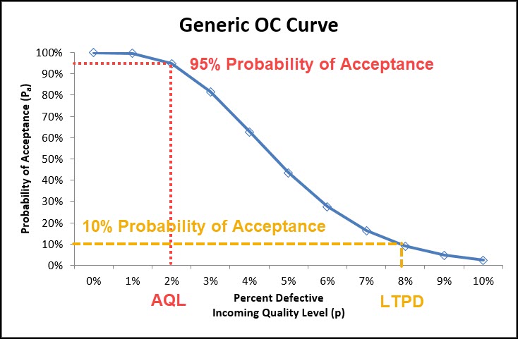
If we look at this OC Curve above, we can tell that the AQL associated with this sampling plan is 2%, and the LTPD for this sampling plan is 8%.
Part 2 – Sampling Standards and Plans
Alright, are you ready for the second part of this chapter which is the actual sampling standards and plans themselves.
This includes a review of basic sampling plans such as single, double, multiple, sequential, and continuous sampling plans.
Then we will review the more complex sampling schemes in ANSI/ASQ Z1.4 and Z1.9 standards. Lastly, we will finish this part with a brief description of the Dodge-Romig sampling tables.
Let’s start with the simple concepts of single sampling plan and double/multiple sampling plans.
Single Sampling Plans
A single sampling plan is the easiest and most common sampling plan.
In single sampling plans, an entire lot is accepted or rejected based on the inspection results of a single sample group of size n, taken from the entire lot (population – N).
Single sampling plans are defined by three parameters:
N = Total Lot Size, n = sample size, c = the acceptance number (derived from AQL)
The total lot size is designed as N, and the Sample Size (n) is the number of samples to be inspected.
I’ll jump ahead to the ANSI/ASQ Z1.4 standard to give you an example of what this looks like in practice.
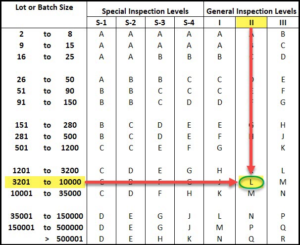
Most normal inspections use General Inspection Level II, and let’s say that your Total Lot Size (N) is 5,000, then your sample size is determined by the Sample Size Code Letter, L.
The Acceptance Number (c) is the maximum number of non-conformances allowed within the sample. The acceptance number is derived from a combination of the AQL you select for the attribute being inspected for, and the sample size.
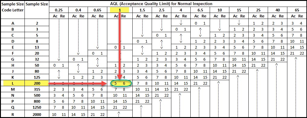
Again, let’s use the ANSI/ASQ Z1.4 standard to demonstrate how to find your acceptance number using your AQL and Sample Size Code Letter.
For this example, let’s say your AQL is 1.0. So, you start by finding your AQL across the top, and your sample size code letter (L in this case) along the side, and you find their intersection in the matrix.
It’s also important to know that this table also specifies the number of samples you should be using during inspection. So you can see that for a sample size code letter of L, you should be inspecting 200 samples (n), and the acceptance number (c) is 5, and the rejection number is 6.
The last key parameter of any sampling plan is the number of non-conformances, d. This is the actual number of non-conformances observed in a sample.
At the conclusion of your inspection of the 200 samples, you would accept the lot if the number of non-conformances found (d) is 5 or less, and you’d reject the lot with 6 or more non-conformances.
The single sampling plan is the simplest to administer and execute, however it results in the largest Average Sampling Number of all the various plans.
If you’re goal is to minimize sampling, you can use the double or sequential sampling plans, which are often able to disposition lots with fewer samples than the single sampling plan.
Double Sampling Plans
While a single sampling plan is executed with only a single sample of units, in double sampling, you can take up to two different samples.
Double sampling plans are effective because oftentimes an incoming lot of product can be so good or so bad that we can make a reasonable conclusion about its quality by taking a sample size much smaller than what is required in a single sampling plan.
Double sampling plans take advantage of this by first taking a smaller sample, then depending on the results, the lot can either be accepted, rejected, or the sampling may continue.
Double sampling plans are defined by n1, c1, r1, and n2, c2, r2. The 1 & 2 subscripts (n1 v n2) simply denote the 1st and 2nd sample.
n = sample size, c = acceptance number, r = rejection number
A lot can be accepted within the 1st sample if the actual number of non-conformances is less than the acceptance number (c). Similarly, a lot can be rejected if the actual number of non-conformances is greater than the reject number.
If the number of non-conformances observed is greater than that the 1st acceptance number (c1) but less than the 1st rejection number (r1) then the sampling continues with the second sample, n2.
Double Sampling Example
Let’s say you want to turn that previous example into double sampling, using the same AQL and starting with the same lot size.
If the overall lot size (N) does change, then the sample size code letter also won’t change, L.
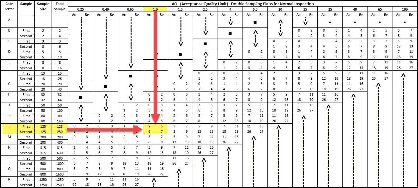
Executing this sampling plan means taking the initial sample (n1) of 125 units and inspecting for non-conformances.
Let’s review quickly how to respond to the various outcomes of this first sample:
- If 2 or fewer non-conformances (c1, acceptance number) are found in this initial 125 units, then the entire lot is accepted.
- If 5 or more non-conformances (r1, rejection number) are found in this initial 125 units, then the entire lot is rejected.
If, let’s say three non-conformances is found in this initial 125 units, then we move on to the second sample of another 125 samples (n2).
Then the results of both samples are combined to make a final decision, so let’s review those possible outcomes:
- If, a combined total of 7 non-conformances are found between both samples (250 total), then the lot is rejected.
- If, a combined total of 6 (or fewer) non-conformances are found between both sample groups, then the lot is accepted.
Remember, the final decision at the end of the second sample is cumulative. You must combine the non-conformances found in the first and second sample and compare that against r2.
Multiple Sampling Plans
A multiple sampling plan is simply an extension of the double sampling plan, where sampling can go on for up 7 to different samples.
Similar to the double sampling plan, each sample taken has its own accept(c) and reject (r) requirements.
Let’s look at the multiple sampling plan for sample size code letter L, with an AQL of 1.0.
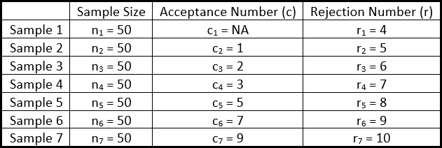
Similarly, to the double sampling plan, over time, these plans have shown to have a lower average sampling number (ASN), when compared to a double or single sampling plan.
The downside is that it these plans can be difficult to administer and create waste (muda) in the form of excess motion when picking samples.
Sequential Sampling Plans
The sequential sampling plan is a further extension of the multiple sampling plan where sampling can go on indefinitely until the entire lot is inspected.
Neither ANSI/ASQ Z1.4 or Z1.9 have sequential sampling plans.
ANSI/ASQ Z1.4 – The Attribute Sampling Plan
The ANSI/ASQ Z1.4 standard is acceptance sampling for attribute data and originated as Military Standard 105.
This standard applies to processes that are continuous in nature, and do not apply to processes that operator infrequently or irregularly.
The Z1.4 standard allows the user to choose between single, double, or multiple sampling plans, and then assists the user in setting up their sampling scheme.
Since we’ve already discussed the nuances of the single, double, multiple and sequential plans, let’s focus now on the sampling schemes and switching rules within the ANSI/ASQ standard.
A sampling scheme is a set of sampling plans that are used along with switching rules that govern with sampling plan should be used. These various sampling plans include normal sampling, heightened sampling and reduced sampling.
These switching rules are integral to the standard.
Many people simply use various sampling plans with no switching rules. This is not the intention of the standard.
The intention of the standard is to be used as a system that uses the switching rules. If you’re not using the switching rules, you’re not inspecting per ANSI Z1.4.
These sampling schemes are meant to reward vendors who have demonstrated a stable, high quality process with reduced sampling, and encourage continuous improvement for poorly performing vendors with heightened sampling.
Let’s jump into the standard itself and discuss how to use it specifically.
The ANSI standard has 3 general inspection levels (I, II and III), and 4 special inspections, which you can see below.
The special inspection levels should only be used when small sample sizes are necessary due to high inspection costs. These small sample sizes naturally result in large sampling risks for both the producer and consumer. Using these special plans must come with an assessment, and acceptance of those risks.
We’re going to focus mainly on the general inspection levels within the standard.
Normal sampling starts with General Inspection Level II, this should be the default starting point for any sampling plan or scheme.
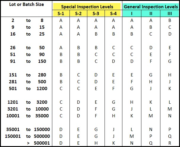
As you can see in the table above, moving between inspection level I, II and III changes the sample size code letter, which changes the number of samples associated with a sampling plan.
For example, if your lot size is 100,000 units, here are the sample size code letters and sample sizes:
- Level I translates to a sample size code letter L, which has a sample size of 200
- Level II translates to a sample size code letter N, which has a sample size of 500
- Level III translates to a sample size code letter P, which has a sample size of 800
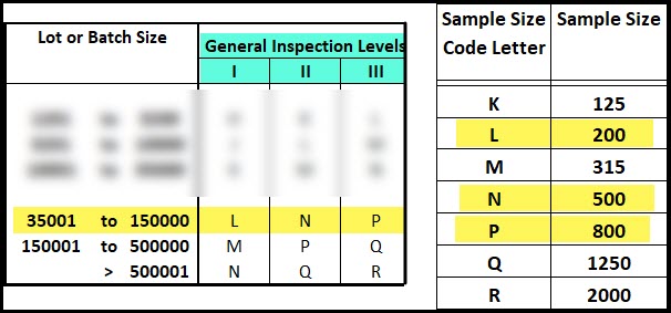
While these different inspection levels might all have the same AQL, Inspecting more samples always reduces the consumers risk of accepting a bad lot. So General Inspection Level I may be used when more risk can be tolerated, and General Inspection Level III may be used when less risk can be tolerated.
A Sampling Scheme
Let’s review the details associated with switching between heightened, normal and reduced sampling inspection.
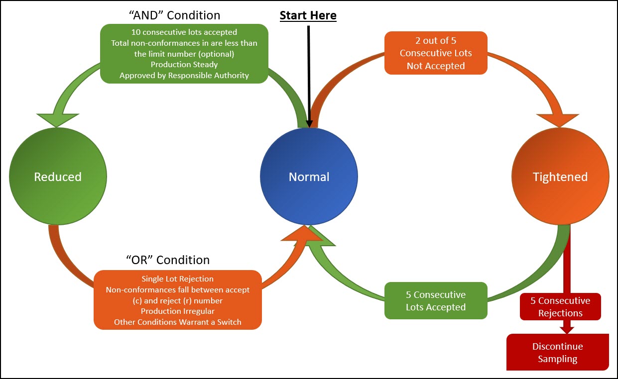
All sampling schemes should start with Normal Inspection.
Reduced inspection is a set of plans that have a reduced sample size compared to normal inspection. Reducing the sample size increases the consumer risk, however this risk can be tolerated due to the strong performance of the supplier.
Tightened inspection is a set of plans that have the same sample size, but a lower acceptance number and rejection number to reduce the consumer risk.
Below is a comparison of the sampling plans for Normal, Heightened and Reduced for an AQL of 1.0. This shows both the sample sizes and accept/reject numbers for each.
I’ve highlighted in purple the difference in sample sizes between reduced and normal inspection. I’ve also highlighted in yellow the difference in the accept/reject numbers between normal and heightened inspection.
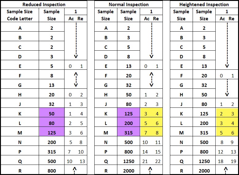
You may also notice that some of the reduced sampling plans have lower accept/reject numbers. This is to ensure the same AQL for the smaller sample size.
The last comment about reduced sampling is if the number of actual rejects falls between the accept/reject number, the lot is accepted, however the plan switches away from reduced sampling back to normal inspection.
There is also a fourth condition within the switching scheme that is worth mentioning which is discontinued sampling.
If an incoming lot has been on tightened inspection and has 5 consecutive rejection, the entire sampling methodology can be discontinued which moves the incoming material to 100% inspection. Sampling cannot resume until the vendor has taken corrective actions to improve the stability or capability of their process.
Let’s discuss what’s requires to switch between these different sampling inspection plans.
Switching Rules
Normal to Tightened
As I said above, sampling schemes always starts with normal inspection. Switching from normal sampling to tightened sampling should occur when 2 out of 5 consecutive lots are rejected. This is an indication that the supplier needs to improve the stability or capability of their process.
Tightened to Normal
A vendor can come off of tightened inspection and move back to normal inspection after 5 consecutive lots being accepted.
Normal to Reduced
To go from normal sampling to reduced sampling all of the follow conditions must be met:
- 10 consecutive lots accepted
- The total number of non-conformances in the previous 10 lots is less than the “Limit Numbers” than the Limit Number found in Table VIII in the applicable standard. If using double or multiple sampling, all inspected should be considered.
- Production is at a continuous and steady rate
- Reduced sampling is acceptable, desirable and approved by the responsible authority
Reduced to Normal
A sampling scheme should switch from reduced inspection to normal inspection if any of the following conditions occur:
- A single lot is rejected
- If the number of non-conformances (d) is between the acceptance number (c) and the rejection number (r). In this scenario, the lot is accepted, but reduced sampling is discontinued.
- The supplier’s production process is irregular or infrequent
- Other conditions warrant a switch
ANSI/ASQ Z1.9 – The Variable Sampling Plan
The ANSI/ASQ Z1.9 standard is acceptance sampling for variable data (to estimate the lot percent non-conformances), and originated as Military Standard 414.
The advantage of using variable data is that the sample sizes are much smaller when compared to attribute sampling, while still offering the same level of protection against consumer and producer risks.
The disadvantage is in the administration of the plans where the math is complex.
These sampling plans are based on the assumption of normality, and they use descriptive statistics like the average, range and standard deviation to make inferences about the overall population.
Similar to Z1.4, Z1.9 is based on a switching scheme where product can switch between normal, reduced or tightened inspection based on the incoming quality from the supplier. The switching criteria within Z1.9 closely reflects those in Z.14.
Additionally, Z1.9 also has plans for single, double and multiple sampling plans.
Variable sampling often requires comparison of sample statistics (average and standard deviation) against both an upper and lower specification to estimate the overall percentage of non-conforming material in lot. This also increases the complexity and administrative costs associated with the variable sampling plan.
Recall that the Attribute sampling standard (Z1.4) allows you to group various quality characteristics into a single sampling plan. This standard is applicable only to the measurement of a single quality characteristic. If multiple quality characteristics must be evaluated, the administrative costs associated with variable plan increases.
This standard provides 3 different calculation processes for sampling based on 3 different estimates of the Lot Variation.
- When the standard deviation is known.
- When the standard deviation is unknown and the average range is used to estimate the Variation.
- When the standard deviation is unknown and the sample standard deviation is used to estimate the Variation.
This standard also provides 5 different inspection levels which can be used. 3 levels of General Inspection (I, II and III) and 2 levels of Special Inspection (S3 & S4). Similar to the Z1.4 standard, the default inspection level is general level II.
I’m not including any tables or example calculations for the variable sampling plans as they are used less frequently and are outside the scope of this text.
Part 3 – Sample Integrity
It’s not an understatement to say that the samples we take during acceptance sampling are very important.
Because of this, it’s important to take care when pulling these samples to ensure that they are representative of the overall population, and not subject to any biases or unnecessary risks.
Specifically, randomness in the sampling process is critical. This ensures that the sample is representative of both the central tendency and variation associated with the overall population.
Not properly randomizing the sample process can result in bias (lack of accuracy) associated with your data, which can have a major impact on the final disposition (accept/reject) of the product.
The goal of random sampling is to ensure that every item in the population has an equal chance of being selected for the sample.
For example, if you wanted to determine the average home price in America by taking a sample, your data would be very biased (lacking accuracy) if you only called homeowners who lived in Manhattan or Hollywood.
Of if during the sampling of incoming parts, you only pulled parts from the box on the top of the pallet. These boxes might represent the end of the run from the vendor which might have performed differently than the start of the run.
Sampling without replacement is another important topic when using double/multiple sampling. Sampling without replacement means that when taking multiple groups of samples, you must not return the tested product back into the general population of product.
Conclusion
Whew! Done! If you made it this far, congrats.
Okay, let’s recap.
Acceptance Sampling is a practice whereby a sample is tested from a population (lot), and a decision to accept or reject that entire population (lot) is based on the test results of the sample.
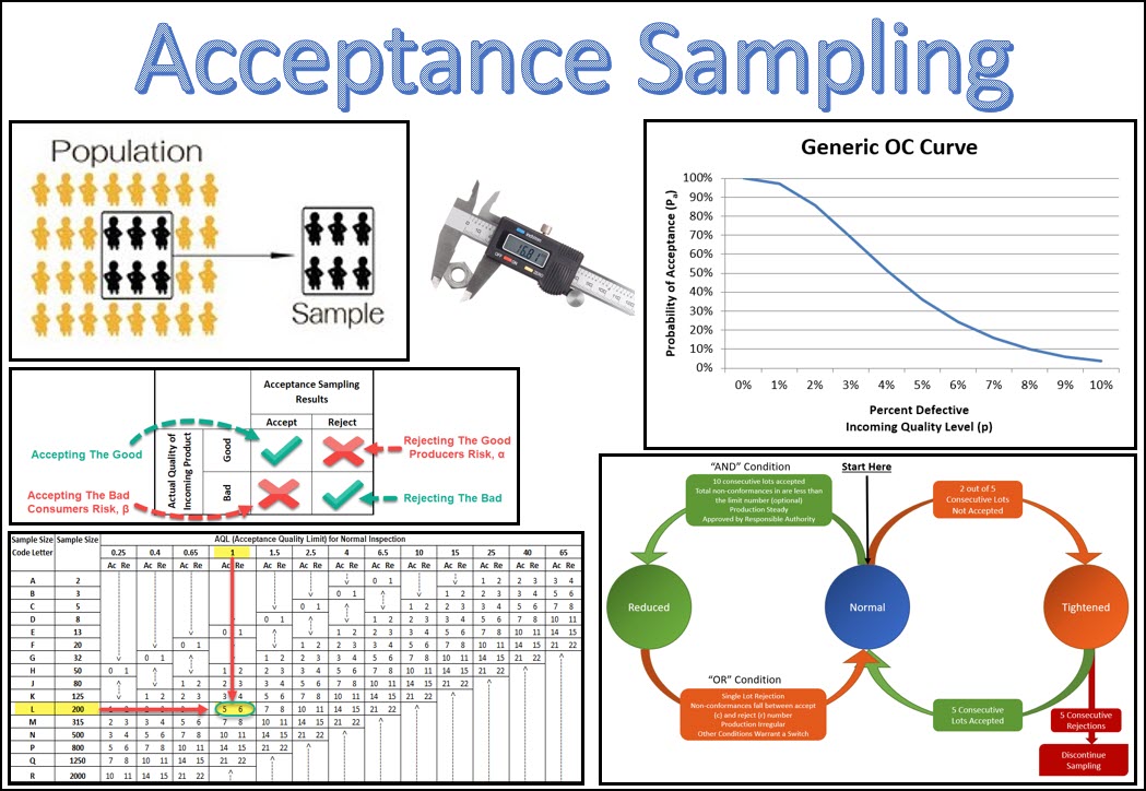
This chapter had 3 major parts.
The first part was the fundamental sampling concepts.
This includes topics such as the operating characteristic (OC) curve, producer and consumer risk, and discussion of common sampling terms like AQL, LTPD, AOQ, and AOQL.
The second part was the sampling standards and plans.
This includes a review of ANSI/ASQ Z1.4 and Z1.9 standards, an explanation of single, double, multiple, sequential, and continuous sampling plans, and a review of Dodge-Romig sampling tables.
The third part was sample integrity, which included a discussion of the techniques for establishing and maintaining sample integrity when executing a sampling plan.