There are three kinds of lies: lies, damned lies, and statistics. – Benjamin Disraeli
We’re about to move into the fun part of statistics – Inferential Statistics, and I’m super excited!
Inferential statistics is a collection of tools & techniques that allow us to draw conclusions about populations based on information obtained from sample data.
The best place to start in Inferential statistics is with the basic concept of Estimators.
There are two types of estimators, Point Estimates & Interval Estimates, and we will discuss the similarities & differences between these two within the chapter.
From a very basic perspective these two tools allow you to estimate population parameters (mean, variance, etc) using data taken from a sample.
I’ll say that again. . .
We’re using sample data to estimate a population parameter.
This chapter is laid out in two sections, the first is dedicated to the Point Estimate, and the second is for the Interval Estimate.
Within the Point Estimate section of this chapter we will:
- Review the concept of Populations & Samples
- Discuss the Point Estimate for the Population Mean, Population Variance & Standard Deviation,
- Discuss the concept of an Unbiased & Efficient Estimates &
- A review of the concept of Standard Error
Within the Interval Estimate Section we will:
- What is a Confidence Interval
- Confidence Intervals for the Population Mean
- Confidence Intervals for Population Variance & Standard Deviation
- Confidence Intervals for Proportions
Populations, Samples & Inferential Statistics
Ok, so we’ve discussed the fact that inferential statistics is a collection of methods that allow us to make inferences about a population based on information obtained from a sample of data.
So let’s jump into that and cover some of these key terms and look at their definitions so that you’re crystal clear on what we’re doing here.
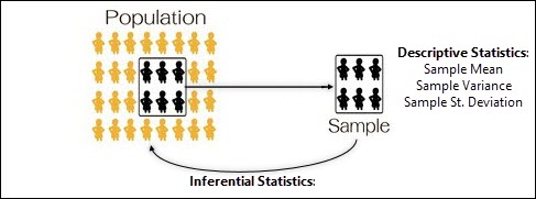
Within statistics, a population is defined as a total set of objects, events or observations about which you want to study.
In quality engineering we’re often interested in knowing the mean & standard deviation associated with populations we’re dealing with.
However, we rarely have the time or resources to measure all values associated with our populations, which is where sampling helps us.
A Sample is defined as a unique subset of a population.
You can see that in the image below where we have a population of people, and we’ve taken a sample from that population.
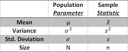
Recall back to chapter two on Statistics (Collecting & Summarizing Data Part 2) where we discussed the difference between a Statistic & a Parameter.
When we talking about sample data and we calculate the mean or standard deviation, we are calculating a Statistic.
Statistics are associated with samples.
When we’re talking about the entire population – the population mean or population standard deviation, we’re talking about a Parameter.
Within the table below you can see the common Population Parameters & their associates sample statistics.
Parameters, Statistics & Estimates
In inferential statistics, we take our sample data and we calculate our sample statistics.
We can then use those sample statistics to estimate the population parameter; which is often times what we’re really looking to understand.
These sample statistics are used within this concept of an estimate, where there are two types of estimates, Point Estimates & Interval Estimates.
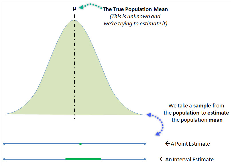
A point estimate is a type of estimation that uses a single value, oftentimes a sample statistic, to infer information about the population parameter as a single value or point.
An interval estimate is a type of estimation that uses a range (or interval) of values, based on sampling information, to “capture” or “cover” the true population parameter being inferred.
The likelihood that the interval estimate contains the true population parameter is given by the confidence level.
You can see both of these estimates below.
The top of the image is the population distribution, with the true population mean shown, which is the population parameter that we’re attempting to estimate.
This population mean can be estimated by a single point estimate, or as an interval estimate.
Point Estimates
Ok, let’s quickly jump into the first type of estimate, the Point Estimate.
A point estimate is a type of estimation that uses a single value, oftentimes a sample statistic, to infer information about the population parameter.
Let’s go through some of the major point estimates which include point estimates for the population mean, the population variance and the population standard deviation.
Point Estimate for the Population Mean
So let’s say we’ve recently purchased 5,000 widgets to be consumed in our next manufacturing order, and we require that the average length of the widget of the 5,000 widgets is 2 inches.
Instead of measuring all 5,000 units, which would be extremely time consuming and costly, and in other cases possibly destructive, we can take a sample from that population and measure the average length of the sample.
As you know, the sample mean can be calculated by simply summing up the individual values and dividing by the number of samples measured.

Example of Sample Mean Calculation
Calculate the sample mean value of the following 5 length measurements for our lot of widgets: 16.5, 17.2, 14.5, 15.3, 16.1

Point Estimate for the Population Variance & Standard Deviation
Similar to this example, you might want to estimate the variance or standard deviation associated with a population of product.
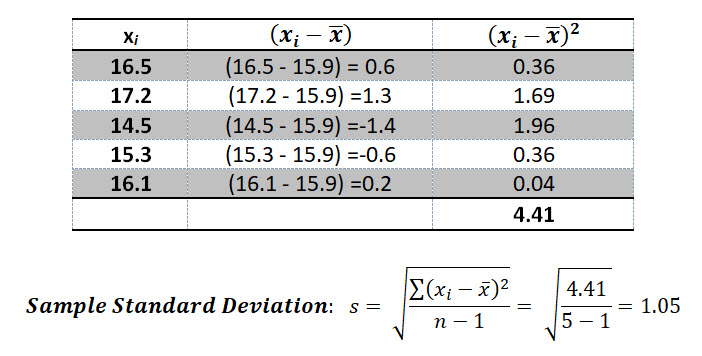
The point estimate of the population variance & standard deviation is simply the sample variance & sample standard deviation:

Example of Sample Standard Deviation
Let’s find the sample standard deviation for the same data set we used above: 16.5, 17.2, 14.5, 15.3, 16.1
Make sense? Now let’s switch on to a few important topics before jumping into the confidence interval section.
Unbiased & Efficient Estimators
Anytime we’re using an estimator to infer a population parameter, you will naturally incur some risk (or likelihood) of inferring incorrectly.
Then entire field of Inferential statistics, by nature, involves a certain element of risk, which we will talk a lot about over the next few chapters.
So to minimize the risk associated with estimators, we desire two characteristics of a high quality estimator, that they are unbiased & efficient.
Unbiased
An unbiased estimator is one who’s expected value is equal to the population parameter being estimated.
Consider the situation where we are repeatedly sampling (sample size = n) from a population distribution.
Each sample would have its own distribution of values, which are all shown under the main population distribution.
Let’s say you sampled 100 units from a population of 1,000 and you calculated the sample mean.
Based on the random nature of sampling, you’d expect each sample taken to likely have a different sample mean.
Now let’s say you repeated this sampling 30 times; and you plotted the distribution of sample means.
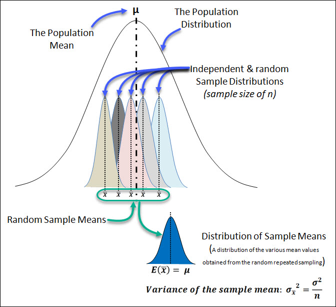
This new distribution of sample means has its own variance & expected value (mean value).

A point estimate (the sample mean, in this example) is considered unbiased if it’s expected value is equal to the parameter that it is estimating.
Bias & Variance
This same thing can be said for the sample variance (S2), in that the expected value of the sample variance can be shown to be equal to the population variance (σ2).
A quick caveat about that here, if you compare the equation for Population Variance against the Sample Variance, you’ll notice they have different denominators.

The population variance is divided by N, while the sample variance is divided by n-1, this is to account for bias.
If you calculated the sample variance using only N, you’d find that the estimate tends to be too low and therefore biased.
This is why we divide by n-1 as this has been shown to be an unbiased estimate of the population variance.
Efficiency
The second characteristic of a high quality estimator is one that is efficient and it is a reflection of the sampling variability of a statistic.
When it comes to estimating a population parameter like the population mean, there can often be many ways to estimate that population mean.
A more efficient estimator is one that has the lowest variance (sampling variability) associated with it.
For example, to estimate the population mean you could use two different estimators.
The first estimator could be the sample mean, while the second sample could simply be a single observation from the population as an estimate.
To pick the more efficient estimator between these two options (sample mean v. a single observation) we must understand the variance associated with each estimator.
The variance of a single observation is simple, it’s equal to the population variance σ2 .
The variance of the sample mean distribution is:

If we compare these together we can see that the variance of the sample mean is smaller than the variance of a single observation.

Therefore we can conclude that the sample mean is a more efficient estimator of the population mean than a single observation because it’s variance is lower.
For the population mean, we measure the efficiency (sampling variability) of our sample using the Standard Error.
Standard Error
As discussed above, whenever we create a distribution of sample means, that distribution of sample means will also have a certain amount of variability to it.
This is a reflection of the efficiency (sampling variability) associated with our sampling (size of n). The smaller the standard error, the less sampling variability.
Within the context of this chapter, we’re only going to discuss the standard error associated with the sample mean distribution.
With some statistics work that’s out of scope of this text, we can prove that the variance of the sample mean distribution:

The Standard Error of a this sample mean distribution is analogous to the Standard Deviation in that it is a reflection of the dispersion or spread of sample mean values around the population mean.
Similar to the standard distribution, the Standard Error is the square root of the sample mean distributions variance.

The Standard Error is equal to the population standard deviation, divided by the square root of n.
We will use this concept of the standard error in the next section when we discuss the confidence interval. This standard error is also called the margin of error.
Confidence Interval (The Interval Estimate)
An interval estimate is a type of estimation that uses a range (or interval) of values, based on sampling information, to “capture” or “cover” the true population parameter being inferred / estimated.
Interval estimates are created using a confidence level, which is the probability that your interval truly captures the population parameter being estimated.
Because we use a confidence level, we often call these interval estimates a confidence interval.
You can see an example of the confidence interval below.
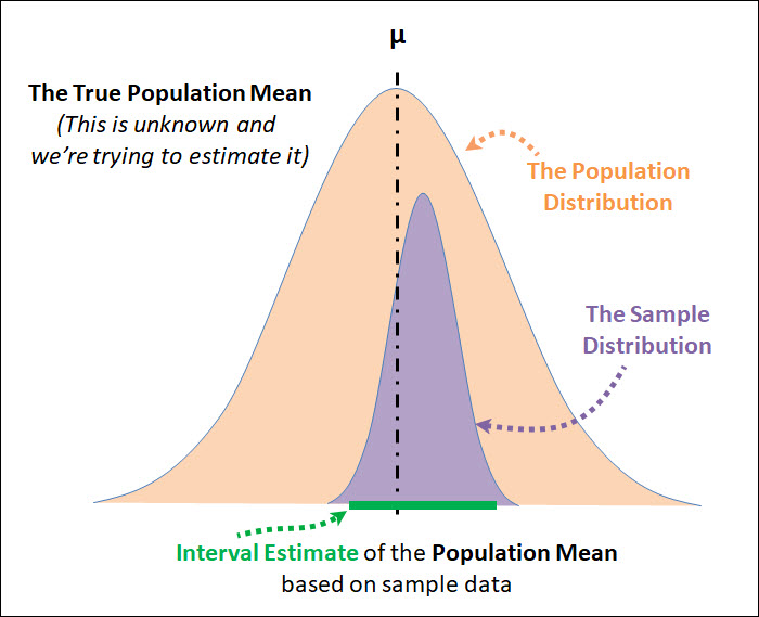
The image starts with the population distribution in orange, and this distribution has an unknown population mean, which we’re attempting to estimate.
Then we take a sample (of size n) from that population, and that sample distribution is shown in purple.
We can then create our confidence interval based on that sample data.
Let’s talk more about this confidence level before jumping into the interval calculations.
What does a Confidence Level Mean?
The confidence level is an often miss-understood concept.
When we say that we have 95% confidence in our interval estimate, we do not mean that 95% of the overall population falls within the confidence interval.
The confidence level is the probability that your confidence interval truly captures the population parameter being estimated.
So if we have a 95% confidence level, we can be confident that 95% of the time (19 out of 20), our interval estimate will accurately captures the true parameter being estimated.
If you look at the graph below, the true population parameter (μ in this case) is shown as the solid blue line down the middle.

In 19 of the 20 intervals created, the true population mean is captured within those 19 intervals. There is only 1 interval that does not capture the true population mean and it’s shown in red.
Up until this point I’ve only used the 95% confidence level, but your confidence level can vary.
You can be 80% confident, 90%, 99% ,etc.
The confidence level you choose is based on risk – specifically your alpha risk (α).
Alpha risk is also called your significance level and it is the risk that you will not accurately capture the true population parameter.
Your Confidence Level then is equal to 100% minus your significance level (α).
Confidence Level = 100% – Significance Level (α)
So if your significance level is 0.05 (5%), then your confidence level is 95%.
The Confidence Interval Equation
Ok, similar to the confidence level, I wanted to start by talking generically about the confidence interval equation, so that you understand the different components.
Once you get this part, the various situations (Mean, variance, proportion), is just an adaptation of this equation.
The confidence interval equation is comprised of 3 parts: a point estimate (also sometimes called a sample statistic), a confidence level, and a margin of error.
The point estimate, or statistic, is the most likely value of the population parameter and the confidence level & margin of error represents the amount of uncertainty associated with the sample taken.
Confidence Interval = Point Estimate + Confidence Level * Margin of Error
When dealing with the population mean, the confidence interval looks like this:

You’ll notice that the margin of error for the population mean is equal to the standard error discussed above.
The standard error can be impacted by the sample size (n) associated with your sample, where a larger sample means a smaller margin of error. The margin of error is also impacted by the standard deviation.
The Confidence Level & Z-Score
You’ll notice in the example above, the confidence level is expressed as a Z-score that also references the alpha risk (Significance level).
In this situation, we’re using the Z-score because the distribution of sample means is normally distributed.
Essentially what this confidence level is doing is capturing a certain proportion (95% for example) of the sample mean distribution when creating the interval estimate.
In the various other situations, where we’re creating a confidence interval for variance & standard deviation, that data follows the chi-squared distribution.
So those confidence intervals use the Chi-squared value instead of the Z-score.
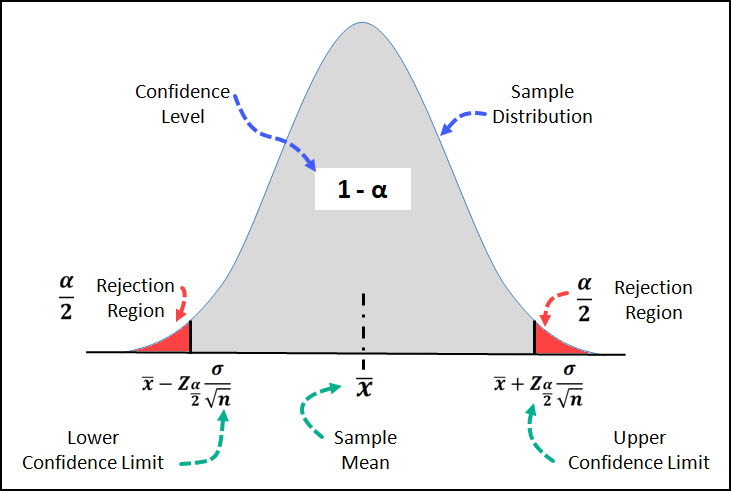
On this graph you can see that the region shaded in gray in the middle captures a certain portion of the distribution, for example if your confidence level is 95%, it would capture 95% of the distribution.
The region in red is often called the rejection region, but I’ve shown it that way to demonstration the alpha risk.
The alpha risk, 5% in this example, is split in half between the left and right tail of the sample distribution which is why the equation and the image show it as α/2 .
In this example the sample distribution is the normal distribution, but in other interval estimates we might be using the t-distribution or the chi-squared distribution.
Confidence Interval for the Population Mean
Ok, time to jump into the meat of the confidence interval discussion and show you the actual equations.
Ok, so when it comes to creating an interval estimate for the Population Mean, there are two possible equations.
These two possible equations are based on whether or not the population variance is known or unknown.
When the population variance is known, you use the normal distribution (z-score) and the population variance to create your interval estimate using the following equation:

When the population variance is unknown, you use the t-distribution (t-score) and the sample variance to create your interval estimate using the following equation:

I’ve highlighted the difference between the z-score and t-score above in red, and I’ve highlighted the difference between the sample variance & population variance in blue.
Another way to decide between the equations above is based on the sample size n.
Generally, if the sample size is less than 30, the t-distribution should be used. If the sample size is greater than 30, then the normal distribution can be used.
Let’s do an example of each.
Example of Interval Estimate of Population Mean with Known Variance
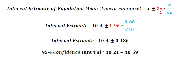
You’ve sampled 40 units from the latest production lot to measure the weight of the product, and the sample mean is 10.40 lbs. If the population standard deviation is known to be 0.60 lbs, calculate the 95% confidence interval.
Ok, let’s see what we know after reading the question:
n = 40, σ = 0.60 lbs, α = 0.05, x-bar = 10.4 lbs.
Before we can plug this into our equation we need to find the Z-score associated with the 95% confidence interval.
If we look that up in the NIST Z-Table, we find Z = 1.96.
The Z-score of 1.96 is associated with an area under the curve of 0.475.
This is because the normal distribution is two-sided and the alpha risk associated with one side of the distribution is 0.500 – 0.025 = 0.475.
Example of Interval Estimate of Population Mean with Unknown Variance
You’ve measure 10 units from the latest production lot to measure the length of the product.
You calculate the sample mean to be 17.55 in, and the sample standard deviation to be 1.0 in.
Calculate the 95% confidence interval for the population mean.

Ok, let’s see what we know after reading the problem statement:
n = 10, x-bar = 17.55 in, s = 1.0 in, α = 0.05.
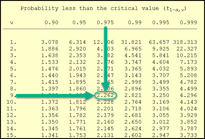
Before we can plug this into our equation we need to find the t-score associated with the 95% confidence interval.
With n = 10, we can calculate our degrees of freedom (n – 1) to be 9.
Since this confidence interval is two-sided, we will split our alpha risk (5%) in half (2.5% or 0.025) to lookup the critical t-value of 0.975 (1 – α/2) in the NIST t-distribution table at 2.262.

Let’s switch gears now and jump into the confidence intervals for the Population Variance & Standard Deviation.
Confidence Interval for the Population Variance & Standard Deviation
Similar to the mean, it’s often the case in inferential statistics that we want to use sample data to estimate the population parameter of Variance or Standard Deviation.
Below are those equations, which are identical except for the square root that’s taken for the standard deviation.
One key difference with this equation when compared against the ones above for the population mean, is that these confidence intervals are not symmetric.
This lack of symmetry is caused by the underlying distribution, the chi-squared distribution.
This confidence interval is also based on the alpha risk (significance level), and that alpha risk is used in conjunction with the chi-squared distribution.

Example of a Confidence Interval for the Population Standard Deviation
You’ve taken a sample of 10 units from the latest production lot, and measured the overall length of the part.
You calculate the sample mean to be 17.55 in, and the sample standard deviation to be 1.0 in.
Calculate the 95% confidence interval for the population standard deviation.
n = 10, s = 1.0 in, α = 0.05, x-bar = 17.55
First we must find our critical chi-squared values associated with our alpha risk and sample size, let’s do that first.

I’ve highlighted the two chi-squared values associated with the confidence interval:
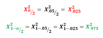
Now we can go to the NIST Chi-Squared Table and look up those critical values for the degrees of freedom of 9 (n-1):
 Now we can complete the equation using these chi-squared values along with the sample size, and sample standard deviation to calculate our interval.

Confidence Interval for Population Proportions
Alright, on to the topic here for Confidence intervals, and that’s confidence intervals for Proportions.
The confidence interval equation for the population proportion is very similar to that of the population mean.

This interval uses 3 different variables:
- Critical Z score associated with the alpha risk

- p = the sample proportion
- n = sample size
In other textbooks you’ll see the sample proportion called p-hat; this is to distinguish it from p which is also often used to represent the population proportion.
Example of Confidence Interval for Population Proportions
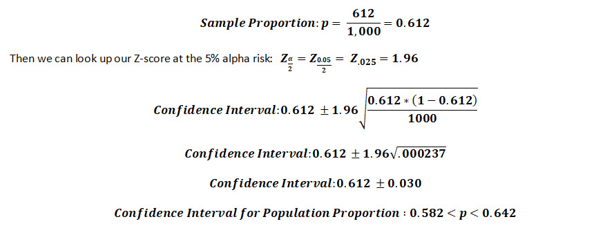
You’ve surveyed 1,000 individuals from your neighborhood to determine how many of them would be willing to pay a higher Homes Owners Associated fee in order to build a neighborhood pool. 612 said yes.
Find the 95% confidence interval for the true population proportion for your neighborhood.

This interval uses 3 different variables:
- Critical Z score associated with the alpha risk

- p = the sample proportion
- n = sample size
First we can calculate the sample proportion, p using n = 1,000 and 612 “yes” votes:
Conclusion
Inferential statistics is a collection of tools & techniques that allow us to draw conclusions about populations based on information obtained from sample data.
We started in on Inferential Statistics with the basic concept of Estimators, and there are two types of estimators, Point Estimates & Interval Estimates.
This chapter is laid out in two sections, the first is dedicated to the Point Estimate, and the second is for the Interval Estimate.
A point estimate is a type of estimation that uses a single value, oftentimes a sample statistic, to infer information about the population parameter as a single value or point.
The sample mean, sample variance, sample standard deviation & sample proportion are all point estimates of their companion population parameter (population mean, population variance, etc.)


We also discussed the two characteristics of a high quality estimator, that is an estimator that is unbiased & efficient.
An unbiased estimator is one who’s expected value is equal to the population parameter being estimated.
An efficient estimator is one that has the lowest variance associated with it when compared to other potential estimates.
We then jumped into the 2nd half of the chapter to discuss interval estimates.
An interval estimate is a type of estimation that uses a range (or interval) of values, based on sampling information, to “capture” or “cover” the true population parameter being inferred.
Interval estimates are created using a confidence level, which is the probability that your interval truly captures the population parameter being estimated.
We then reviewed the confidence interval for the population mean, both when the variance was known and unknown:

We then reviewed the confidence interval for the population variance & standard deviation:

Lastly, we reviewed the confidence interview for the population proportion.
